In machine learning and statistics, feature selection, also known as variable selection, attribute selection or variable subset selection, is the process of selecting a subset of relevant features (variables, predictors) for use in model construction.
Feature Selection is a technique in which we want to decrease the number of features keeping the performance of our model same (or increasing it). It is a common perception in ML community that garbage in garbage out, so if we input noise in out model then our model is gonna return dubious outputs. So we want to create a minimal feature set from our existing feature set.
First we calculate the collinearity between a single feature and target variable (should be maximum) and we use different filter methods to calculate these collinearity:
Notation
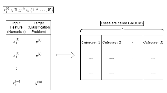
$x^{(i)}$ denotes the input variables , and $y^{(i)}$ denotes the output or target variable that we’re trying to predict, where the superscript $“(i)”$ denotes the $i^{th}$ training sample.
Note that the superscript “(i)” in the notation is simply an index into the training set, and has nothing to do with exponentiation.
A pair $(x^{(i)},y^{(i)})$ denotes a single training example.
$x^{(i)} \in \mathbb{R}^n$, i.e., $x^{(i)}$ is $n$ dimensional, while $y^{(i)} \in \mathcal{C}$.
$x^{(i)}_j$ represents the $j^{th}$ feature of the $i^{th}$ training sample.
$m$ denotes the number of training examples.
$n$ denotes the number of features.
The entire training data is denoted as $\mathcal{D} = \lbrace ({x}^{(1)},y^{(1)}), \cdots, ({x}^{(m)},y^{(m)}) \rbrace \subseteq \mathbb{R}^n \times \mathcal{C}$.
The data points $(\mathbf{x}_i,y_i)$ are drawn from some (unknown) distribution $P(X,Y)$. Ultimately we would like to learn a function $h$ such that for a new pair $(\mathbf{x},y)∼P$, we have $h\mathbf{(x)}=y$ with high probability (or $h(\mathbf{x})≈y$). We will get to this later. For now let us go through some examples of $X$ and $Y$.
In terms of computation, they are very fast and inexpensive and are very good for removing duplicated, correlated, redundant features but these methods do not remove multicollinearity. Selection of feature is evaluated individually which can sometimes help when features are in isolation (don’t have a dependency on other features) but will lag when a combination of features can lead to increase in the overall performance of the model. The list of different filter methods that can be used are classified below:
We will discuss the important methods below:
Analysis Of Variance (ANOVA)
The correlation between a numerical and categorical variable is find using statistical test such as F-test (ANOVA), t-test, etc. In this case, we will use ANOVA for hypothesis testing.
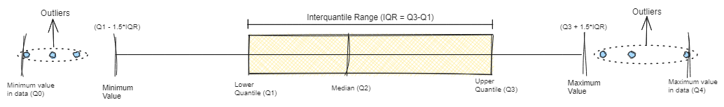
ANOVA stands for Analysis Of Variance. So, basically this test measures if there are any significant differences between the means of the values of the numeric variable for each categorical value. This is something that you can visualize using a box-plot as well. A typical box-plot is shown below with five number summary:A typical box-plot with important notations
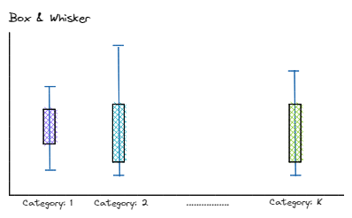
The below items must be remembered about the ANOVA hypothesis test. The definition of the group is defined as follows:'A feature is disintegrated according to the classesAnd using the box plot we can visualize the distribution according to each category:Box-plot for each class
Null hypothesis $H_0$:
There is no relationship between independent variable and dependent variable (basic definition)
The variables are not correlated with each other.
Groups means are equal (no variation in means of groups)
Alternate hypothesis $H_0$:
There is a relationship between independent variable and dependent variable
The variable are correlated with each other.
At least, one group mean is different from other groups
We then calculate the mean for all groups: The proof will be presented later but remember that we have an important identity as:
$$SS_{total} = SS_{within-group}+SS_{between-group}$$
where $SS$ represents “Sum of Squares”. After that we create what we call an ANOVA table:
$$\begin{array}{c:c:c:ccccc}
\text{Source} & \text{(DoF)} & SS & \text{Variance} \\ \hline
\text{within-group} & N-K & SS_{within-group} & \frac{SS_{within-group}}{N-K} \\ \hline
\text{between-group} & K-1 & SS_{between-group} & \frac{SS_{between-group}}{K-1} \\ \hline
\text{Total} & N-1 & SS_{total} & \frac{SS_{total}}{N-1}
\end {array}$$
The term F-test or F-statistic is based on the fact that these tests use the F-values to test the hypotheses. An F-values is the ratio of two variances.
Variances measure the dispersal of the data points around the mean. Higher variances occur when the individual data points tend to fall further from the mean. Here’s the F-value for one-way ANOVA.
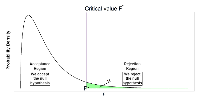
Now, we have calculated the F-value, what we need to do is find the critical value using the F-distribution curve, The F-distribution table is organized based on the $\alpha$ value (usually 0.05). Next, the columns of the f-distribution table are based on df1 (degree of freedom for numerator or between-group) while the rows are based on df2 (degree of freedom for denominator or within-group).
F-distribution curve
Now, we have find the F-critical and F-value, then we can find whether to accept the null hypothesis or reject the null hypothesis.
Chi-square test for Categorical Features
The chi-square statistics is a way to check the relationship between two categorical nominal variables.
Nominal variables contains values that have no intrinsic ordering. Examples of nominal variables are sex, race, eye color, skin color, etc. Ordinal variables, on the other hand, contains values that have ordering. Examples of ordinal variables are grade, education level, economic status, etc.
Pearson’s chi-squared test is used to assess three types of comparison: goodness of fit, homogeneity, and independence.
A test of goodness of fit establishes whether an observed frequency distribution differs from a theoretical distribution.
A test of homogeneity compares the distribution of counts for two or more groups using the same categorical variable (e.g. choice of activity—college, military, employment, travel—of graduates of a high school reported a year after graduation, sorted by graduation year, to see if number of graduates choosing a given activity has changed from class to class, or from decade to decade).
A test of independence assesses whether observations consisting of measures on two variables, expressed in a contingency table, are independent of each other (e.g. polling responses from people of different nationalities to see if one’s nationality is related to the response).
For all three tests, the computational procedure includes the following steps:
Define your null and alternative hypotheses before collecting your data. (In our case, the null and alternative hypotheses are same from the ANOVA hypothesis testing)
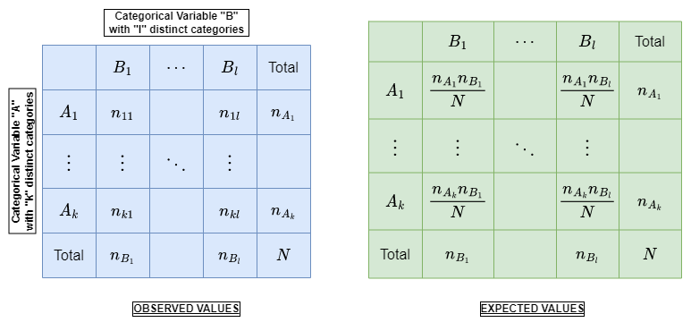
Calculate the chi-square test statistics, using the contigency table. Here is how you create a contigency table and calculate the chi-square value using the contigency table:Contigency TableTherfore, the chi-squared statistics is calculated as follows:
$$\chi^2=\sum_{i=1}^{N}\frac{(O_i-E_i)^2}{E_i}=\sum_{i=1}^{N}\frac{O_i^2}{E_i}-N$$
Determine the degrees of freedom, df, of that statistic.
For a test of goodness-of-fit, df = (number of categories - 1)
For a test of homogeneity, df = (number of rows − 1)×(number of Cols − 1), where Rows corresponds to the number of categories (i.e. rows in the associated contingency table), and Cols corresponds to the number of independent groups (i.e. columns in the associated contingency table).
For a test of independence, df = (number of rows − 1)×(number of Cols − 1), where in this case, Rows corresponds to the number of categories in one variable, and Cols corresponds to the number of categories in the second variable.
Select a desired level of confidence (significance level, p-value, or the corresponding alpha level) for the result of the test.
Compare the obtaines chi-square value to the critical value from the chi-squared distribution with df degrees of freedom and the selected confidence level (one-sided, since the test is only in one direction, i.e. is the test value greater than the critical value?)
Now, we have find the chi-square-critical and chi-square-value, then we can find whether to accept the null hypothesis or reject the null hypothesis.
The above method is one form of chi-square test known as Pearson chi-square test. There are other chi-square test as well such as Yates’s correction for continuity, phi coefficient, contigency coefficient, Cramer’s V, etc. The definition of these are:
$$\chi_{yates}^2=\sum_{i=1}^{N}\frac{(|O_i-E_i|-0.5)^2}{E_i}$$
$$\phi=\pm \sqrt{\frac{\chi^2}{N}}$$
$$C=\sqrt{\frac{\chi^2}{\chi^2+N}}$$
$$V=\sqrt{\frac{\chi^2/N}{min(k-1,l-1)}}$$
Mutual Imformation based Correlation
Mutual information is a concept from information theory and statistics that measures the amount of information that two random variables share. It quantifies the degree of dependency or association between the variables. In simpler terms, mutual information tells us how much knowing the value of one variable can help us predict the value of another variable.
Mutual information (MI) between two random variables is a non-negative value, which measures the dependency between the variables. It is equal to zero if and only if two random variables are independent, and higher values mean higher dependency. Mutual Information methods can capture any kind of statistical dependency, but being nonparametric, they require more samples for accurate estimation.
Consider two random variables $X$ and $Y$ with a joint probability mass function $p(x,y)$ and marginal probability mass functions $p(x)$ and $p(y)$. The mutual information $I(X;Y)$ is the relative entropy between the joint distribution and the product distribution $p(x)p(y)$
If the natural logarithm is used, the unit of mutual information is the nat. If the log base 2 is used, the unit of mutual information is the shannon, also known as the bit. If the log base 10 is used, the unit of mutual information is the hartley, also known as the ban or the dit.
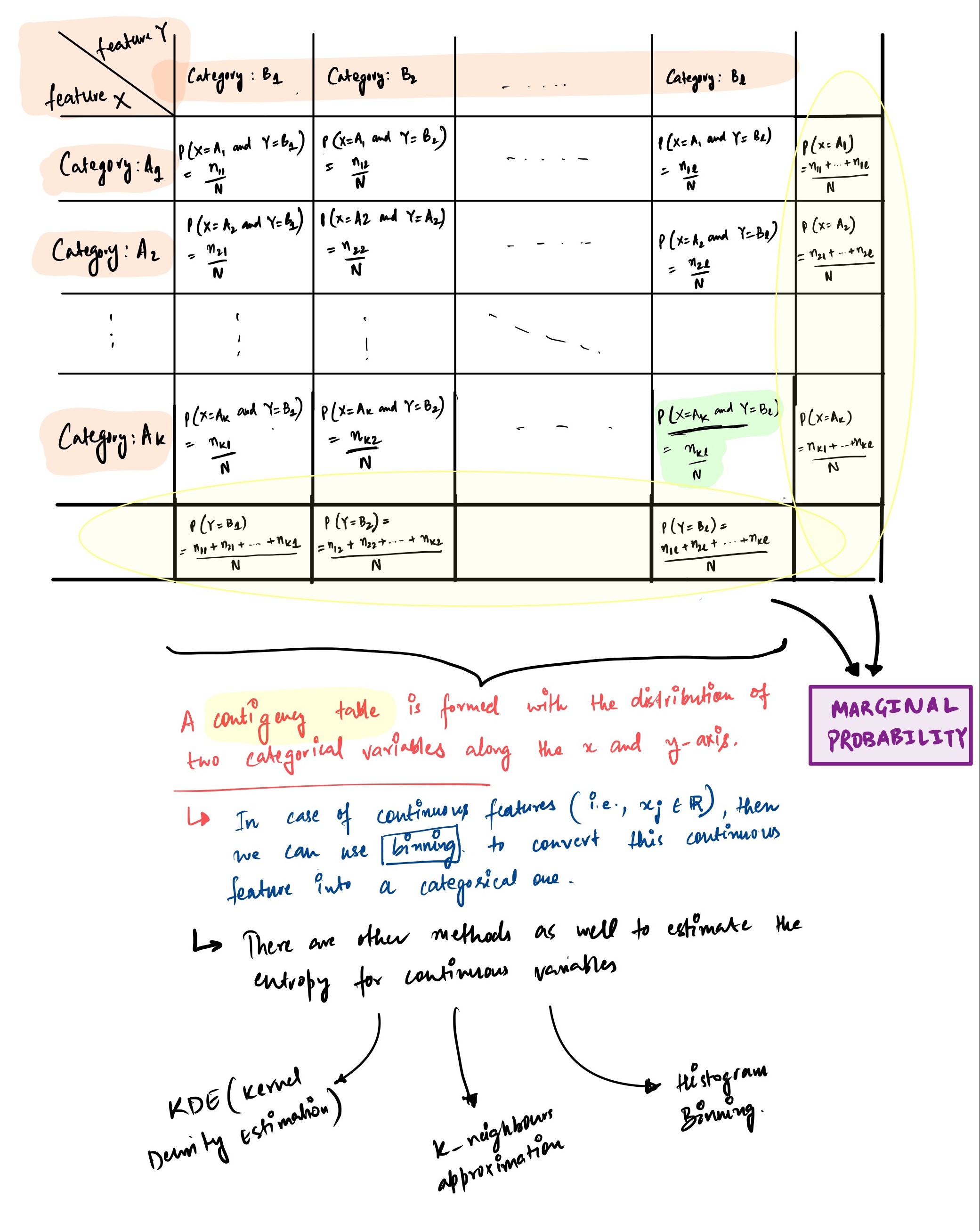
The current approach for calculating mutual information for two categorical features is given by:
We have $X \in {x_1,x_2,\cdots,x_K}$ and $Y \in {y_1,y_2,\cdots,y_L}$ are two categorical features with $X$ having $K$ categories and $Y$ have $L$ categories.
Make a contingency table from the variables.
Normalize the table so it all sums to 1. This would approximate the joint distribution $p(x,y)$.
Use this to compute mutual information.
Mutual Information
The above methods computes the Mutual Information given both the random variables are categorical if any of the variable is numerical, then we have to convert that continuous variable into discrete variable. In order to do so, there are various methods, the simplest one is binning. Another method that is quite popular is nearest neightbour method of entropy estimation between continuous and discrete variable. I haven’t provided the description of that method, but there are several papers implementing that approach.
Normalized Mutual Information:
If you want to use Mutual Information as an indicator of how strongly two variables correlate, it is useful to normalize into a range of [0,1]. The most intuitive way of doing this might be:
This would be the uncertainty coefficient (Theil’s U).
Univariate Analysis - Correlation Coefficient
The correlation value (correlation coefficient) is used to measure the strength and nature of the relationship between two continuous variables (numerical variables) while doing feature selection for machine learning. The value ranges between -1 and +1. A correlation of -1 shows a negative correlation, while a correlation of 1 shows a perfect positive correlation. A correlation of 0 shows no linear relationship between the movement of the two variables.
Pearson correlation coefficient (named after Karl Pearson) is used to show a linear relationship between two variables. It is calculated as:oefficient $(r)$
Pearson correlation coefficient (named after Karl Pearson) is used to show a linear relationship between two variables. It is calculated as:
$$
r=\frac{\sum (x_i- \bar{x})(y_i- \bar{y})}{\sqrt{\sum (x_i- \bar{x})^2 \sum (y_i- \bar{y})^2}}
\\
r=\text{correlation coefficient}
\\
x_i=\text{values of the x variable in a sample}
\\
\hat{x}=\text{mean of the values of the x variables}
\\
y_i=\text{values of the y variable in a sample}
\\
\hat{y}=\text{mean of the values of the y variables}$$
There are some assumptions relating to the usage of the Pearson-R correlation coefficient:
Both variables should be normally distributed (gaussian distribution)
Linearity: Linearity assumes a straight-line relationship between each of the two variables
Homoscedasticity: Homoscedasticity assumes that data is equally distributed around the regression line
Spearman Correlation Coefficient $(\rho)$
Spearman correlation (named after Charles Spearman) is the non-parametric version of Pearson’s correlations. The Spearman correlation evaluates the monotonic relationship between two continuous. In a monotonic relationship, the variables tend to change together, but not necessarily at a constant rate. The Spearman correlation coefficient is based on the ranked values for each variable rather than the raw data.
Similar to Pearson’s Correlation, Spearman also returns a value between [-1,1] for full negative correlation and full positive correlation, respectively.
Comparison between Pearson and spearman Correlation coefficient
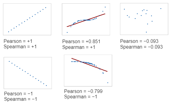
There are some problems with these correlation coefficients. One is the presence of outliers and the other is that these correlation coefficients can handle only the linear relationship. Pearson correlation coefficients measure only linear relationships. Spearman correlation coefficients measure only monotonic relationships. So a meaningful relationship can exist even if the correlation coefficients are 0. Examine a scatterplot to determine the form of the relationship.
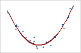
This graph shows a very strong relationship. But the Pearson coefficient and Spearman coefficient are both approximately 0.